Why Laplace transforms are so useful

In this exploration of the Laplace transform, we begin with a physical simulation: a mass on a spring influenced by an external, oscillating force—much like a gust of wind blowing back and forth. When left alone, the spring has a natural frequency at which it wants to oscillate. However, when an external force is applied at a different frequency, the system behaves strangely at first. It produces an irregular, "wibbly" startup trajectory, growing stronger and weaker before eventually settling into a steady, predictable rhythm. To analyze this behavior and predict how long it takes for the system to find its stride, we utilize one of the most powerful tools in engineering and physics: the Laplace transform. The Laplace transform acts as a translator, moving a function from the domain of time into the "s-plane." This s-plane represents all possible values of a complex number, $s$, which sits in the exponent of functions like $e^{st}$. In this language, the vertical imaginary axis represents oscillation, while the horizontal real axis represents growth or decay. Specifically, poles—points where the transformed function blows up to infinity—reveal the "exponential pieces" hidden inside a system’s behavior. If a pole has a negative real part, the system decays toward zero; if it has a positive real part, the system is unstable and explodes. If it has an imaginary component, the system oscillates. 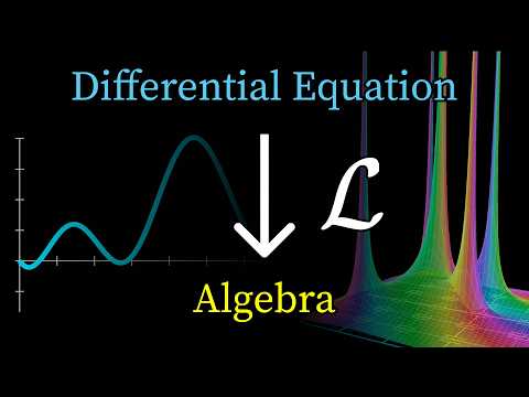The true utility of the Laplace transform lies in its ability to convert complex differential equations into manageable algebra. This is made possible by a specific mathematical property: the transform of a derivative. When you take the Laplace transform of a function's derivative, it is equivalent to multiplying the transform of the original function by $s$, and then subtracting the value of the function at time zero. This "minus $f(0)$" term is not a nuisance; it is a vital feature that builds initial conditions—like starting position or velocity—directly into the algebraic process. To see this in practice, consider the simple harmonic oscillator: a mass on a spring with damping (friction). The physical forces involved are proportional to the mass's position and its velocity. When we add an external oscillating force, such as a cosine wave, the resulting differential equation becomes significantly harder to solve using traditional methods. However, by applying the Laplace transform to every term in the equation, the calculus vanishes. The second derivative of position becomes a term involving $s^2$, the first derivative involves $s$, and the position itself remains a constant. This process transforms the left side of our differential equation into a quadratic polynomial—a "mirror image" of the original physical system. If we assume the system starts from rest, the initial condition terms drop out, leaving us with a clean algebraic expression. On the right side of the equation, the external cosine force is also transformed into an expression with poles on the imaginary axis at its specific frequency. By dividing the system’s polynomial into the force’s transform, we obtain a complete description of the system’s dynamics in the s-domain. Even before we translate this back into the time domain, the s-plane tells the whole story. The final expression has four poles. Two come from the spring system itself; these usually have negative real parts, meaning the "natural" vibration of the spring will eventually decay and disappear. The other two poles come from the external force and sit directly on the imaginary axis, meaning they represent a persistent oscillation that never dies away. This explains the "startup" period seen in the simulation: the irregular wibbling is the result of the natural frequency and the external frequency competing. Once the natural frequency decays due to damping, only the external frequency remains, and the system hits its steady-state stride. To find the exact mathematical solution, one would use partial fraction decomposition to break the complex fraction into simpler pieces and then invert the transform. Each simple fraction corresponds to an exponential term in the time domain. For those interested in the underlying mechanics of the system—such as preventing a bridge from wobbling to ruin—the key is to analyze how the amplitude of the final oscillation changes as the external frequency approaches the natural resonant frequency of the system. Finally, we must ask why the derivative property works. There are three ways to view it. The first is through a specific example: applying the transform to $e^{at}$ and using algebraic manipulation to show that the result indeed matches the $s \cdot F(s) - f(0)$ formula. The second is the formal textbook approach using integration by parts, which provides a rigorous proof but can sometimes obscure the intuition. The third and most profound explanation involves the inverse Laplace transform. This involves the idea that the Laplace transform and its inversion are a unified pair designed specifically to turn differentiation into multiplication. This deeper theory involves contour integrals and links the Laplace transform to the Fourier transform. Understanding how to reinvent these tools from scratch allows us to see that the Laplace transform is not just a clever trick for solving homework problems, but a fundamental framework for understanding how any dynamic system evolves over time.