The Physics of Euler's Formula | Laplace Transform Prelude

This lesson serves as the foundation for understanding the Laplace transform by focusing on the behavior of exponential functions, specifically in the form $e^{st}$. Here, $t$ represents time and $s$ is a parameter that determines the specific nature of the exponential. To understand the transform, one must first master the mental framework of how these functions behave when $s$ is allowed to be a complex number. The starting point is the fundamental property of $e^t$: it is its own derivative. While derivatives are often visualized as slopes on a graph, a more dynamic approach is to view them as velocity. If $e^t$ represents the position of a point on a number line, the derivative tells us that the velocity is always equal to the current position. Starting at 1, the point moves right, and as its position increases, its velocity increases, leading to accelerating growth. If we change the exponent to $e^{2t}$, the velocity is twice the position, causing even faster growth. Conversely, with a negative exponent like $e^{-0.5t}$, the velocity is half the position but pointed in the opposite direction, resulting in exponential decay toward zero. 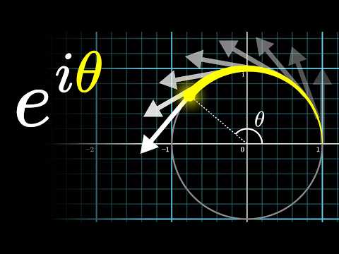The behavior becomes most interesting when $s$ is an imaginary number, such as $i$. Using the chain rule, the derivative of $e^{it}$ is $i$ times the function itself. Geometrically, multiplying a complex number by $i$ corresponds to a 90-degree rotation in the complex plane. This means the velocity vector is always perpendicular to the position vector. The only motion satisfying this condition is a constant rotation around a circle. This explains why $e^{it}$ traces a unit circle over time, and why $e^{\pi i}$ equals -1, as $\pi$ units of time bring the point halfway around the circle. This leads to the concept of the "S-plane," where every point represents a different exponential function $e^{st}$. The imaginary part of $s$ (often denoted as $\omega$) controls the angular frequency or how fast the function oscillates. The real part of $s$ determines whether the function grows or decays. A negative real part combined with an imaginary part creates a trajectory that spirals inward toward the origin, a visual representation of decaying oscillation. These mathematical properties are essential for solving differential equations in physics, such as the motion of a mass on a spring. The position of the mass, $x(t)$, is governed by Newton’s Second Law, where the force is proportional to the displacement (the spring constant $k$) and the velocity (the damping coefficient $\mu$). This results in a linear differential equation: the sum of the mass times acceleration, the damping force, and the restoring force equals zero. A common, albeit "bizarre," trick to solve such equations is to guess that the solution takes the form $e^{st}$. When you substitute $e^{st}$ into the differential equation, every derivative term simply pulls down a factor of $s$. Because the exponential term itself is never zero, it can be factored out, leaving a quadratic polynomial in $s$. Solving this polynomial—known as the characteristic equation—reveals the values of $s$ that make the original differential equation true. In a system with no damping, the roots for $s$ are purely imaginary, representing a perfect, perpetual oscillation. When damping is introduced, the roots gain a negative real component, reflecting the physical reality of a spring that eventually settles to a stop. If the damping is high enough, the roots become purely real, representing an "overdamped" system that decays without oscillating at all. Because these equations are linear, we can combine multiple exponential solutions. If we find two complex solutions, we can scale and add them together to produce a real-valued solution that matches physical reality. This principle of linearity allows us to satisfy specific initial conditions, such as the starting position and velocity of the mass. While this "guessing trick" works for simple linear equations with constant coefficients, real-world physics often involves more complexity, such as an external forcing term. For example, in optics, charges in a material act like damped oscillators driven by the external oscillation of an incoming light wave. In these cases, simple guessing is insufficient. This is where the Laplace transform becomes necessary. It systematizes the idea of breaking down complicated functions into their "atomic" parts: the exponentials $e^{st}$. The Laplace transform translates a function from the time domain into a new language where these exponential components are the fundamental units. In this new domain, the operation of differentiation in time is transformed into simple multiplication by $s$. Consequently, difficult differential equations are converted into straightforward algebraic problems. By viewing functions as combinations of points on the S-plane, engineers and physicists can analyze growth, decay, and oscillation through a unified lens, turning the calculus of change into the algebra of exponents.